
Punch line: hazard events have the potential to introduce significant dispersion in projected cash-flow streams and, commensurately, the modeling and valuation of risky projects.
Investing in risky projects where projected cash-flows are subject to significant disruption, contingent on stochastic events, involves modeling and pricing for the inherent uncertainty. The following stylized illustration provides a rudimentary simulation-based valuation framework where geo-hazard events (earthquakes, volcanoes, floods etc.) have the potential to significantly disrupt the“base-case” projected cash-flow stream.
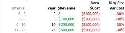
To set the stage, assume the following “base-case” 4-phase revenue-cost curve; 3 transition states (year 0-2, 3-5 and 6-10) and a final steady state to maturity (year 11-25). Cost are split into fixed costs (lease, rent, equipment, fees, permits, insurance etc.) and variable costs (100% – gross margin %). These assumptions are reflected in the table below:
Next, in order to introduce the potential for geo-hazards to disrupt projected operations, consider small-, medium- and large-scale geo-hazard events with associated probability of annual occurrence and affiliated revenue-cost loss-severity dynamics. These are reflected in the table below:
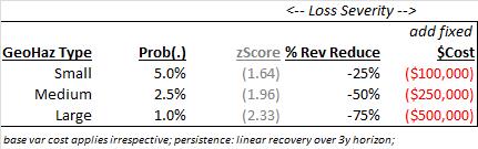
Note: loss severity is assumed to persist over a linearly-dampened 3-year horizon, i.e., if geo-hazard cost (revenue reduction and additional fixed cost) in year j is -$X, then it persists at 2/3 of -$X in year j+1, and 1/3 of -$X in year j+2.
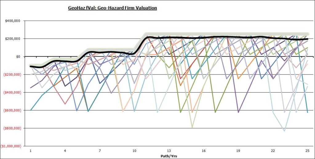
Next, in order to reflect the cash-flow impact of geo-hazard events, populate a 100 by 25 matrix (100 paths of 25 annums each) with random draws from a standardized normal distribution and use that to trigger geo-hazard events, or not, per the specifications above and accordingly simulate annual cash-flows along each path, accounting for the path dependency of prior outcomes. (For e.g. if a random draw is -2.1 then it is treated as a medium geo-hazard event and has the associated loss-severity dynamics (depending on which year/phase it falls) and persists over 3-years in the linearly dampened fashion described above. These cash-flow dynamics are illustrated in the chart below (thick grey high-line reflects modal un-triggered paths; bold black line is the expected-value path, more on this further below):
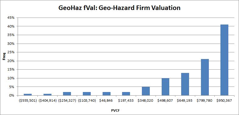
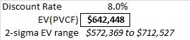
Next, assuming a healthy discount rate (UST 10y + additional risk premium; 8% all-in this illustration), compute the present value of the cash-flows along each path. This is reflected in the frequency chart below with the low-frequency long-left tail highlighting the cash-flow impact of extreme geo-hazard events:
Finally, the average of the present value of the path cash-flow streams represents the potential valuation of this risky investment in a simulation-based risky world (since we’re using the same discount rate along each path – geo-hazards independent of rate structure – this is equivalent to the present value of the average cash-flow stream). Additionally, to illustrate the potential for sampling error, we can also compute the 95% confidence range around the expected valuation (95% of the time the true expected value, population mean, lies between a 2-sigma range).
Using this simulation-based valuation along with the standard no-hazard, base-case cash-flow stream yields conventional IRR:

In summation, the above analysis provides a rudimentary framework for risk-return decision-making under uncertainty and underscores the importance of probabilistic valuation given the potential for hazard events to introduce significant dispersion in projected cash-flow streams.
Note: calculations Risk Advisors
Proprietary and confidential to Risk Advisors